We quite often try to use Friday’s lesson as an opportunity to do some form of extension, enrichment, revision, or any other kind of different activity with our Further Maths students. Having just finished teaching the material on Differential Equations to Year 13, I hoped to find an article that demonstrated their application in the ‘real world’. I figured mathematical ecology might well be the route to go down and after quite a quick search on Google, I came across what seemed to be the ideal paper.
Analysis of the Incidence of Poxvirus on the Dynamics between Red and Grey Squirrels
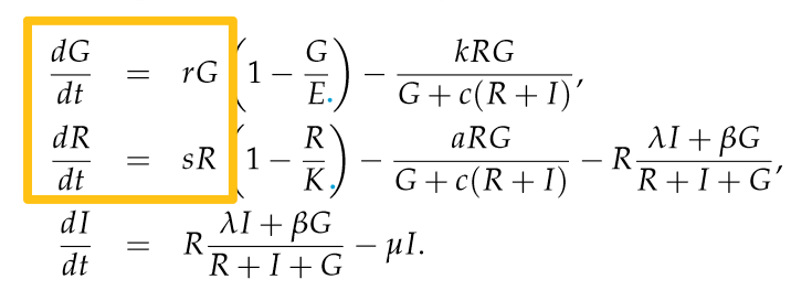
It has a system of 3 coupled differential equations
However, I quickly realised that not only does the initial model get ‘reparametrized’, there are approximately 15 pages of detailed analysis before you get to some discussion of the outcomes.(These pages are occasionally interspersed with some diagrams which at least have a bit of colour to catch the eye!)
How to get anywhere with this and Y13?
Another challenge I considered is that many of my students are non-native English speakers. However, I do know they are willing to trust me and try out activities!
It became clear that I would need to structure the work and focus their attention on key aspects at each step. It then dawned on me that the ability to ‘skim’ an academic paper for the highlights is a somewhat teachable skill.
I (hastily) put together a list of prompts that would guide us through the paper and through the lesson:
The difference between interspecies and intraspecies – a useful pair of prefixes to be able to distinguish
Equilibrium points and if they are stable [demonstrated with a metre ruler: balanced horizontally on two hands it is in equilibrium and stable; balanced vertically on one hand it is (theoretically) in equilibrium but (definitely) not stable!]
Notation for referencing: round brackets referring to equation numbers; square brackets referring to the references
Making sense of the DEs
Whilst the system of differential equations looks rather unpleasant even to me, there are aspects that can be teased out.
The highlighted terms here model a simple growth rate. With no other aspect in the model, both populations would undergo exponential growth which is unfeasible in the long-term.
The newly highlighted terms bring in a factor involving the carrying capacity of the populations. These prevent the long-term population growing without bound as, when G=E or R=K, their rate of population growth will be zero.
Whilst these terms are quite unpleasant to unpick, incorporating the product RG accounts for interactions between the two populations.
Then notice that the final negative term for dR/dt is the same as the first positive term for dI/dt. This is accounting for red squirrels becoming infected and hence their numbers no longer counting for population R but instead for population I.
And, lastly, notice that dI/dt includes a negative term for the mortality rate as a proportion of the size of population I.
Overall…
The students really appreciated doing this activity! And that was for not just its mathematical features (ie noticing the elements of the equations above), and modelling features (appreciating that modelling really does happen, and there are always assumptions and limitations), but also for the guidance of how you can go from the abstract and introduction, take in the equations, and then jump to the discussion or conclusions without necessarily needing to digest anything from the main body of the paper!
With our Y13s gone and our Y12s doing internal exams last week, it’s been a good opportunity for some reflective thinking within our department. This is my first year as HoD (and boy, what a year…) but now I feel settled enough to think about much longer term goals for the department. One of these is to try ‘nudging’ the students’ performance – I guess in a value-added sense – so that students who might be close to grade boundaries can end up on the better side of the fence for example.
Obviously this means identifying some elements of our practice where there is room for further work and improvement. I feel fortunate to have a team who are open to such discussions in department meetings and, individually, enjoy engaging in longer conversations with me whenever we find the time. Whilst I have a scribbled list of half a dozen ideas, here are our (current) top 3. In no particular order…
Corrections
We have (what we believe to be) an effective system in place that includes a relatively hefty weekly homework assignment and also a weekly class test. The homework is very much a formative task and students can access departmental support throughout the week. Indeed, they are also given numerical answers to all the questions and are expected to check, mark and correct their work before the due date. There is no ‘marking’ in the traditional sense – we look to see that students have invested appropriate time and energy in the work and offer constructive feedback on aspects of the work that could improve or, for example, if they’ve used inefficient methods or drawn inadequate diagrams.
With our tests it’s the opposite – these are marked and graded, but we write only the briefest feedback on them. The expectation is that students then follow this up with corrective work (and potentially re-study some aspects of a topic) but we don’t currently have a regular process in place to ensure such follow-up work has happened. We are currently discussing a number of options: should students be asked to resubmit their test at a later date? Should students do all their tests in some kind of exercise book so they and we can always look back and see a longer term picture? Should students keep some kind of reflective list of their errors and misconceptions?
Communication
This idea has already been through several iterations in our discussions. We frequently bemoan the poor presentation, less than logical flow, and generally not quite ‘up to scratch’ nature of our students’ solutions. However, we realise we perhaps don’t have sufficient focus on explicitly teaching our core standards and expectations and then holding students to them.
We are considering a framework for solutions along the lines of “Inputs / Argument / Conclusion”. These names are still evolving but we’re aiming for a common department vocabulary. In brief:
Inputs: this can mean many things in many situations, so some examples might be best. It could be as simple as just copying a pair of simultaneous equations given in a question, adding numbers to them. It could mean a force diagram in Mechanics, summarising all the information presented textually. It could mean a summary of facts about the terms of a sequence, again interpreted from the text of the problem
Argument: this is then the logical flow of the solution with good, correct, clear mathematical communication
Conclusion: this can be the final ‘answer’ (with appropriate rounding and units), a summary statement of what was asked for (eg a clear statement of a binomial approximation, or partial fractions decomposition) etc
Not all of these elements are necessarily present for every question, nor perhaps will they always be clearly disjoint (that isn’t ultimately necessary). But our belief is that clear, careful communication in solutions helps improve students’ prospects of solving a problem fully and correctly.
We are also considering including specific marks in our weekly tests for appropriately meeting these expectations (and thus not simply applying exam-standard mark schemes, that do nothing for improving the quality of students’ responses).
Random revision questions
How often do you present your students with a totally unseen, unrehearsed question on an unexpected topic? For us it is seldom until, for example, we are in revision mode much closer to exams. We are considering a model that perhaps changes from year 12 to 13:
In Year 12… students could be given such a ‘surprise’ exam question once every week or two, as an activity in the classroom. They would try it in exam conditions, but then have the immediate full support of discussion, feedback and correction without any stakes attached. We hope this would highlight to them the need to keep on top of past topics, refreshing their memories every now and again.
In Year 13… such questions could be an element of their weekly test (which is typically rather topic-focussed on recent work). This raises the stakes – weekly test results mean a lot to our students! – but they are that much closer to the end of their course, so we feel it is reasonable to increase the demand.
I had a particularly enjoyable morning with my Year 13s today, eating a chocolate chip muffin and trying out any maths problems we could find online. This led to me discovering a Ukrainian maths textbook and so I thought I’d share some insights and comparisons with what we have in the UK.
Algebra and the beginnings of analysis (Merzlyak et al, 2019) is a textbook for the 11th class, which in Ukraine is the final school year. My understanding is that after the 8th class, students begin to specialise (to some extent) in their subject choices and this book is for those who go down a more mathematical pathway. One of the first things to notice is that the book is recommended by the Ministry of Education and Science of Ukraine.
The book opens with a patriotic and motivational quotation inscribed on a monument to the scientist Kravchuk: My love is Ukraine and mathematics. With the added caption “We hope that this patriotic statement of a prominent Ukrainian mathematician will be a reliable guide for you on the path to professionalism.”
There is an introductory From the authors message, enthusiastically welcoming the 11th class students. They remind students of the need…
“to be persistent, attentive and accurate, and most importantly – do not remain indifferent to mathematics, and love this beautiful science”.
They also point out two additional features of the text: “If after homework there is free time and you want to learn more, we recommend to refer to the section “When the lessons are done”. The material presented there is not easy. But the more interesting to test your strength! In addition to educational material, in the textbook you can find stories on the history of mathematics.” They close by wishing the students success!
Contents & Anatomy
I would assume that the contents of this textbook are a good proxy for the syllabus content for the students’ course. Across 300 pages, we find:
Section 1 (Chapters 1-8; ~80 pages): Exponential and logarithm functions
Section 2 (Chapters 9-12; ~50 pages) Integrals and their application
Section 3 (Chapters 13-19; ~70 pages) Elements of probability theory
The book closes with 40 pages of short answers for all the exercises, an index and a table of contents.
Each chapter comprises a developmental discussion of the theory (including use of the language of ‘lemma’ and ‘theorem’ etc), example problems and then a substantial exercise. For example, Chapter 1 finishes with a set of 52 problems, many of which have multiple sub-parts.
Each section closes with some “When the lessons are done” material and then a summary of the key points covered throughout its chapters. At the end of Section 1, for example, we meet Kravchuk again and learn that he “attached great importance to educational work with young people, in particular, on his initiative in 1935 the first Kyiv Mathematical Olympiad for schoolchildren was held”. The problems from that competition are then included:
Q1 is to evaluate; Q2, 3 are to solve; Q4 is to prove, given that un is arithmetic; Q5 is to prove given (a,b,c) is a Pythagorean triple; Q6 to determine a,b,c such that the quartic is divisible by the cubic
Section 2’s enrichment includes the classic discussion of Newton and Leibniz, but also discusses the much less well-known work of Cavalieri.
Careful development of the theory – a closer look at Chapter 1
The very first chapter, whose primary focus is the function f(x)=ax, discusses briefly what it can mean to raise a number to an irrational power (as the limit of a sequence with rational powers) – something which we, or at least our textbooks, simply take for granted. I wouldn’t say the treatment is quite as rigorous as an undergraduate approach, but it’s nice to see a discussion that uses limits. The language of lemma, theorem and proof is used: eg a lemma is included, proving that “if a>1 and x>0, then ax>1″.
The chapter discussion continues to prove that ax is increasing for a>1, and decreasing for a in (0,1). And even demonstrates its continuity with a limit-of-sequences approach. Also included is the Cauchy functional equation f(x+y)=f(x)f(y) and a discussion about modelling bacterial growth (constant proportional growth over equal time intervals) reduces to this relation, from which we can therefore deduce that the model is exponential. (That Cauchy’s equation implies an exponential function is the final challenge problem at the end of the chapter!)
The thoroughness of the discussion is perhaps also exemplified by the summary table for the function that appears just before the main worked problems and exercise set.
The rows cover: domain, range, zeros, intervals of sign constancy(?), increasing/decreasing, continuity, differentiability, asymptotes
Exercises
A common complaint about many UK textbooks is the paucity of questions to solve. Noticeably here, there is an abundance of practice problems. Chapter 1 ends with a set of 52 problems, many of which have several parts. Moreover, the quantity doesn’t come from repetitive tasks. It feels as if each part of a multi-part question is intended to elucidate a different point.
Whilst the topic of focus driving the exercise is the function ax, the questions cover simplification (numerical and algebraic), graph sketching and considerations of domain and range, inequalities, composite functions (eg 6cos x) and modulus functions, investigating the continuity of given functions etc. The final ten or so questions are marked to indicate their more challenging nature and include solving a system of simultaneous equations, and investigating Cauchy’s functional equation.
This approach of exploring the exponential function from so many angles can only help to strengthen students’ appreciation of the interconnectedness of so many topics which, I fear, our A level books (and perhaps exams) compartmentalise in the extreme.
Class and Homework
This particular textbook uses green to suggest problems that could be set as homework. Interestingly, they frequently seem to appear after a ‘parallel’ question that students will have tackled in class. For example:
Q1.21, 1.22: determine using a sketch how many solutions each equation has. Q1.23, 1.24: sketch. Note a couple of misprints: Q1.24(6) has an erroneous y= and I think Q1.24(4) was intended to be 3-x as per Q1.23(5)
Topics included
I assume the content of the course is prescribed nationally. I’ve already described the textbook contents above and, for example, the complex number work develops into roots of unity, de Moivre’s theorem, and proving trig relationships, much like our A level Further Maths. There is also more extended work on applying complex numbers to geometric problems. The probability chapter includes geometric approaches to tackling some problems.
Also very interesting is the final section, “Polynomials” which covers:
Finding complex roots of eg quadratics (and has a “When the lessons are done” section discussing the ‘lady with the dog’ proof of the fundamental theorem of algebra)
Multiplicity of roots and that higher derivatives equal 0
Viete’s formulae in the cubic case, and Cardano’s approach to solving cubics.
My Top 3
I think the top 3 features of this textbook that I really like are:
Thorough, plentiful exercises that draw together many concepts within one common focus
The questions marked as homework tasks, typically in a very similar style to a preceding problem that students will have had the chance to tackle in the classroom
The extension and enrichment offered in the “When the lessons are done” sections
One to take away
From the probability chapter…
A boy and a girl are meeting for a date sometime between 3pm and 4pm. They can each arrive at any time in that interval, independently of each other. If the boy arrives first, he will wait up to 20 minutes for the girl; if the girl arrives first, she will wait up to 10 minutes for the boy. What is the probability that they will meet?
Each summer I find I have the time to reflect on what is currently working well in my teaching and, importantly, what improvements I might be able to make in the next school year. Of course these improvements should be about making things better for my students, but if they save me time and stress in the long-run then that is also a worthy goal!
With reference to the latest (research-backed) buzzwords that are flying around these days, I’m keen to build in more ‘retrieval practice’. In particular, for my Further Maths classes, I quite often use warm-up questions that bring to the forefront any prior knowledge that the current topic depends on. In my usual style, these were always made up on the fly, but now I am thinking about tightening up on my planning in this area.
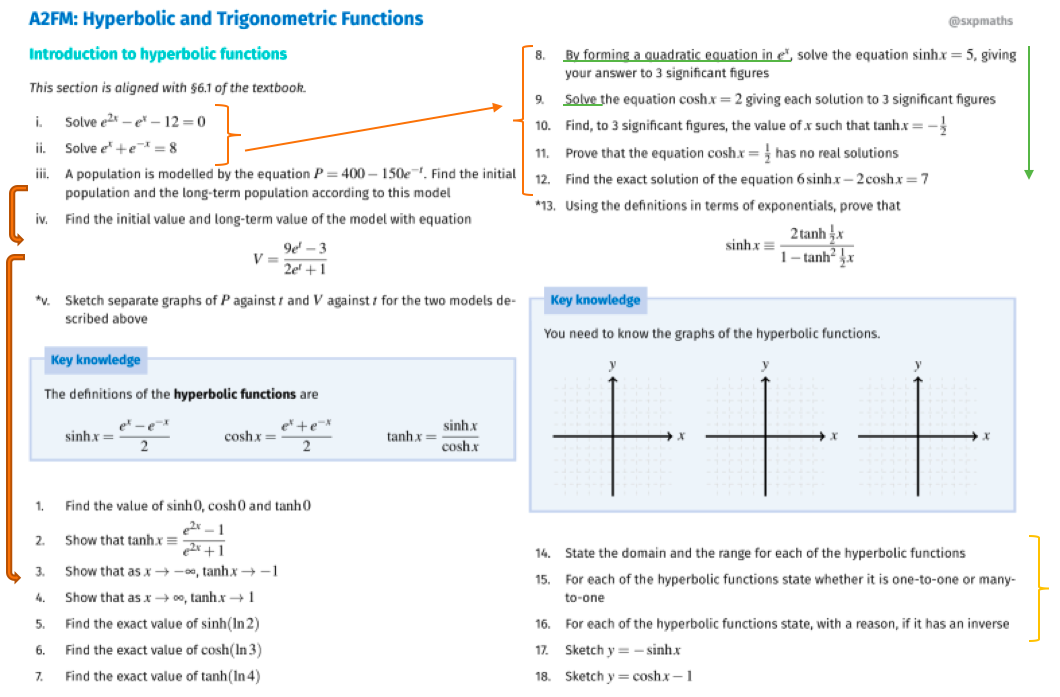
Earlier today on Twitter, I shared a screenshot of the front page of a new style of class sheet that I’m experimenting with, along with a link to access drafts of some of these sheets.
Here is that same screenshot, with additional annotations to help with my explanations below:
Warm-up with a purpose
The questions numbered with Roman numerals are designed to be tackled by the students independently at the very start of a section of study. The intent is that they recap prior knowledge, but with a focus on specific skills that will be called upon in the current section. In my example above, questions (i) and (ii) are clearly designed to remind students about solving ‘hidden quadratics’ of the form that will arise in the subsequent exercise set. Question (iii) brings the concept of a long-term value to the surface and that feeds in to question (iv). The real purpose of these is to understand the behaviour of tanh x in questions (3) and (4) and, indeed, to help us later with graph sketching. Question (*v) is marked with an asterisk, indicating that I don’t expect all students to attempt or fully complete it. (It is there for those who are quick to complete (i)-(iv) and is still useful for those who do tackle it.) In general, questions marked with a * are either optional or more challenging than necessary! In this case, a student who completes question (*v) should have no trouble sketching y = tanh x independently.
Key knowledge
I wanted a way to highlight the most fundamental knowledge for each section of study and opted to do this via the blue ‘key knowledge’ boxes. This information is only presented once and, for example, later warm-up questions ask students to write the exponential definitions down themselves, or sketch the graphs etc – more of that lovely retrieval practice! (My hope is also that these boxes will reduce those annoying, recurring questions in class: “what does the graph of sinh look like again?…” The students will either have a better memory or at least an easy way to look things up.)
Ramped practice
I am not intending these sheets to completely replace the textbook. Ultimately, I find books helpful as a repository of practice questions and indeed a number of my ‘questions’ on the sheet are simply directions to complete specific work from the textbook. However, there are particular skills that I want to highlight and also certain, subtle types of scaffolding that I want to put in place. Thus the questions with Arabic numerals will be a significant part of classwork and I might even choose some to use as examples with the class.
In the screenshot above, I’ve grouped questions 8-12 together as an example of the scaffolded/ramped practice. I phrased question 8 in particular to provide a strong guide to the method of its solution. This scaffolding is then taken away (although, for example, question 9 deliberately says “each solution” to suggest there is more than one). By question 12, students are working at the standard required for this particular skill. Questions like 12 will then pop up in the “warm-up” questions for later sections in this same chapter – more retrieval!
You will likely notice the intention of questions 14-16, too, foreshadowing the next section of work that will look at the inverse hyperbolic functions.
Extension
It’s my intention to end each section with at least one extension question of some sort, although I have not always been able to think of appropriate questions for all sections yet. These will typically come from STEP papers (the STEP database makes it relatively easy to search for problems on a given topic).
Never perfect…
Even with this very first page, I already notice at least one small change that I think would be worthwhile: in the warm-up section I feel it would be good to have a question asking students to simplify e^ln(3) and e^-ln(3) as preparation for questions 5-7.
One of the perennial questions I’m asked (by both students and teachers alike) is “So, where are the answers?”. And I shrug. My own plan is to make much greater use of OneNote next year so that a lot of notes, examples and solutions from class will all be collated in one place. If I make a neat solutions page one day then I’ll be sure to share it, but please don’t hold your breath!
And homework?
Absolutely! I’m a strong believer that homework has value when students are set work within their capability but that includes ‘desirable difficulty’ and, again, a large part of my homework next year will be… retrieval! Our students complete A-level Maths in year 12 before moving on to the FM content in Year 13. I am currently thinking of the following structure for a 10 questions-per-week homework sheet:
3 questions of FM revision (that is, testing topics what were studied 3-4 weeks or more previously*)
3 questions on the current FM topic of study
* our students actually start some FM topics at the end of year 12, so those will form the FM revision section for the early weeks of September
And testing?
Absolutely! Our school policy is actually to have a test every week. In the past I have always focussed these very specifically on the most recent topic of study. However, next year I think they will be structured in a similar vein (and probably corresponding topics) to the weekly homework sheet.
So, what next?
Watch this space, essentially. Over the course of the summer I will be chipping away at the ‘Core Pure 2’ content and tidying up these class sheets. Drafts for three of them are already online but these will be revised again before the summer is out, so don’t rush to download and save them! Also, I’ll be sure to blog again once term has started to reflect on how well (or not) things are going…
It seems, to me at least, that probability is one of ‘those topics’ that students find to be more difficult than others. Each year I have winced slightly as it looms on the horizon of the scheme of work and each year I’ve varied my approach to try and get them (and keep them) on board. This post focusses on conditional probability, now designated as an A-level (not AS) topic.
Prior Knowledge
Students should already have a fair amount of experience with tree diagrams and Venn diagrams. They should also have met the terms independent and mutually exclusive – I think that’s actually where the problems begin. Why are these concepts so challenging? Perhaps because one (independent) is a term borrowed from every day language, but in that standard usage it tends to mean ‘separate from’ which is actually closer to the meaning of mutually exclusive. Secondly, because we try to give students an intuitive and descriptive feeling for what independent means in statistics, they then lose sight of the fact that it has a precise, mathematical definition.
What would I do about this? If I could, I would separate the teaching of the two terms with as much time as possible. We could teach ‘mutually exclusive’ when we cover sampling techniques (the strata for a stratified sample should be mutually exclusive, for example). More contentiously, I wonder if we shouldn’t introduce ‘independent’ until the time we study conditional probability? Compare:
Definition 1: A and B are independent events if
Definition 2: A and B are independent events if
These are equivalent*, but I would argue the second gives a much better feeling for what statistical independence really means.
Conditional Probability
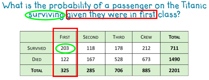
When teaching conditional probability this year, I demonstrated it separately in three contexts: two-way tables, Venn diagrams and tree diagrams. Prior to the discussion of conditional probability, of course I wanted to check that students brought their prior understanding to the surface – through a mixture of starter questions on the board (two-way tables; tree diagrams), or some mini-whiteboard work (Venn diagrams).
In each context I adopted the same approach: a probability question involving the typical ‘given that’ phrasing; a highlighted, restricted part of the diagram; and the formula for conditional probability. Each time, I described the highlighter approach as intuitive and the formula approach as ‘safer’ – not susceptible to misinterpretation. Each time, we also considered the reverse of the conditional statement, ie. we contrasted and .
I split these three contexts over three separate lessons. This gave the students the opportunity to focus on each one fully, in isolation, and to also experience the recall of the formula for conditional probability each day. The examples below aren’t the exact ones that I used in my lessons, but should be illustrative enough.
In a two-way table
Question from LearnZillion
Intuitively:
More abstractly,
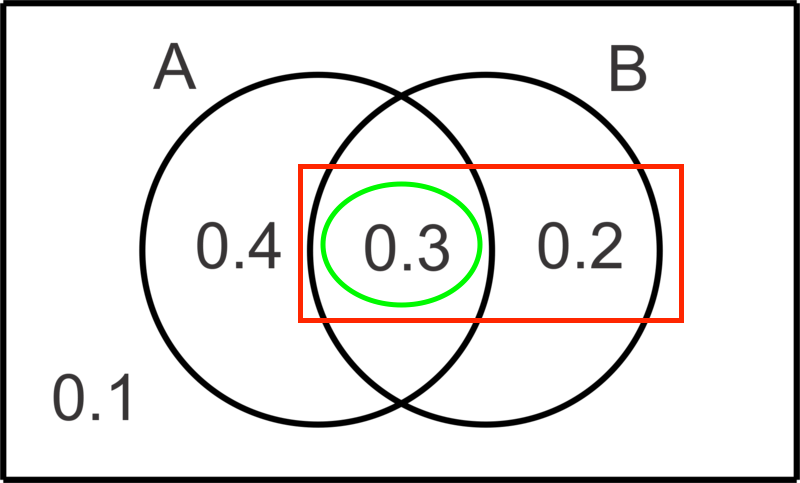
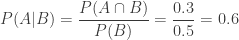
In a Venn diagram
Image from ck12.org
To find , we can think intuitively:
More abstractly,
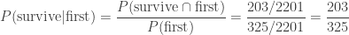
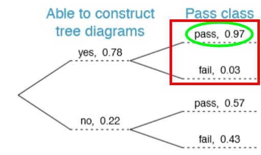
In a tree diagram
Given that a student can construct tree diagrams, what is the probability that they pass? (Image from stats.libretext.org)
Intuitively: just read from the relevant branch.
More abstractly,
Note: there there is a significant opportunity for confusion here: the calculation for is the product , however this is unrelated to the product formula for independent events. Indeed, the events ‘able to construct’ and ‘pass’ are not independent here.
Results and Looking Ahead
We set weekly class tests in our department and thus get fairly rapid feedback about how well students have picked up new topics. I was pleased to see that my emphasis of using the slightly more abstract (but secure) approach given by the formula for conditional probability made an appearance in almost all of the students’ work. I was a little disheartened (but not completely surprised) by the proportion of incorrect answers to the very first question on the test:
1 (a) State what it means for events A and B to be independent.
(b) State what it means for events A and B to be mutually exclusive.
We still have 6 or 7 months to sort that out!
I’ll be returning to conditional probability at every available opportunity. Due to the ordering of our scheme of work, I am now moving on to discrete random variables and thus can include conditional questions there. This is also followed by the binomial distribution (which many of you may well have already taught in the AS year). I find it somewhat surprising that conditional probability has been designed to come after hypothesis testing as, within a hypothesis test, the probability we calculate is conditional on H0 being true. With the order of our own scheme of work, I can emphasise that conditional statement more heavily and hopefully the students will gain a better appreciation for the process we follow in this type of hypothesis test.
* Footnote
The definitions are not quite equivalent… The reason the first is the preferred definition for independent events is that the second cannot be used in the case where . In all other cases, they are equivalent!
One of the new topics to have found its way into Further Maths is coupled systems of differential equations. The Pearson textbook begins with this example:
As both x and y are functions of time, t, then there is a very appealing dynamic nature to the solutions of these equations.
One beautiful way to visualise the family of solutions is to use an online tool called ‘Field Play‘ which I believe was created by Andrei Kashcha (@anvaka). I’ve only been able to capture still images to post here, but the website shows a striking flow over time.
It’s not too hard to enter the equations you wish to visualise, especially once you have seen a couple of examples. The key points are:
v.x represents dx/dt, and v.y represents dy/dt
p.x represents x, and p.y represents y
If you have an integer coefficient (such as 2) then you must enter it as 2.0
Another nice feature of the site is that the settings you enter are encoded in the website link. Thus each link below goes directly to the visualisation of the equations I’ve entered.
Example 1: Bears and Fish
Using the equations from Pearson’s example above yields an image like this:
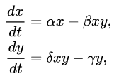
A more sophisticated model for interacting predator and prey species is given by the Lotka-Volterra equations. (Note these are non-linear, because of the xy term, so A level students are not expected to analyse them!)
Here, x represents the population of the prey species, and y the predator.
I found it particularly helpful to project this animation onto my whiteboard so that I could annotate a few features. Note, for example, the location of the origin and labelling of the axes (we were discussing Foxes and Rabbits). The anticlockwise flow follows the typical storyline of alternating fluctuations in predator and prey numbers.
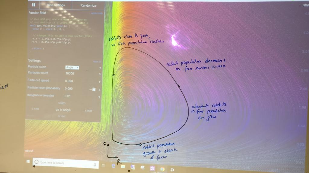
Example 3: Random!
Another great feature of this site is the ‘Randomize’ button. It will generate its own random set of DEs and show you the flow. It can be great to do this several times in succession and notice some features:
These systems have ‘equilibrium points’ where there is no motion. These are points where (simultaneously) dx/dt=0 and dy/dt=0
There are limited types of these equilibrium points: nodes, saddles, spirals, stars etc, and they can either be stable (eg local trajectories spiralling ‘in’ to the equilibrium point) or unstable (spiralling out etc). [A classification based on eigenvalues can be found online in notes such as these.]
The pattern of flow surrounding a number of equilibrium points is strongly reminiscent of weather patterns and might motivate students to learn about Ed Lorenz‘s work on chaos theory.
Proof is one area where the new specifications for A-level Maths are noticeably different from the legacy courses. Technically, proof was a part of the old courses but that box was often ticked by including a trigonometric identity question in exams. MEI gave it a little more prominence with questions like these from their C1 papers:
MEI Core 1, January 2005
MEI Core 1, June 2005
This year I have had to teach proof much more thoroughly than ever before, and it’s certainly not been a straightforward process! This blog post is a reflection on some of the issues that arose and ideas for future teaching.
What’s new?
Each board’s specification contains essentially the same wording when it comes to the content we need to be teaching to cover ‘Proof’ as a topic. Here I’ve copied Edexcel’s specification as it helpfully distinguishes between AS (in bold) and A2, and includes a little bit of exemplification.
Edexcel GCE Mathematics 2017 specification
When I was planning my teaching for this topic, I knew we would need a preliminary discussion about mathematical statements and how they can either be true or false (on a rainy day you might want to disappear down the rabbit hole of incompleteness and Gödel’s work…). I then thought that direct proof by deduction could be done in the same lesson, saving proof by contradiction for a second lesson. Job done. I think it’s fair to use the Bushism that I misunderestimated the depth of this topic!
Lesson 1: warm-up
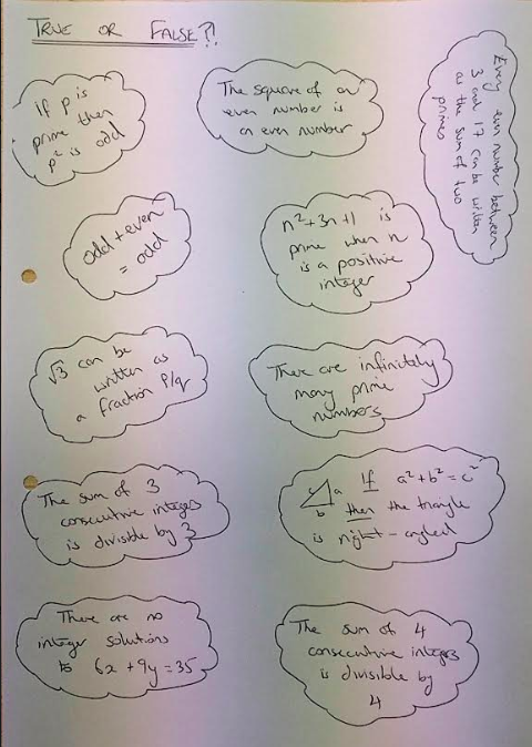
I wrote out a sheet of example statements for paired discussion:
Mathematical prompts for discussion: true or false?
These prompts were designed to include a variety of concepts:
There are rules such as ‘odd+even=odd’ that students have known since junior school, and perhaps have never deeply questioned.
Some of the statements fail in particular instances (the top-left is false when p=2, for example) so we have the notion of a counterexample.
A finite set of cases for checking (top-right) so we have the notion of proof by exhaustion. Which we can then contrast with statements where there are infinitely many cases to check, and thus would need a different approach. [There was also the opportunity to digress and mention Goldbach’s conjecture.]
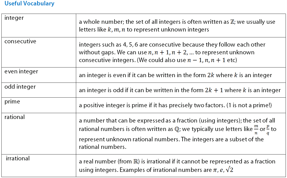
Some statements can be proved using a direct proof by deduction. These will be a nice way to introduce concepts such as writing odd integers in the form , where
I included the converse of Pythagoras so that we could talk about the direction of an implication. Here, the converse is itself a true theorem but that is not always the case.
My other choices are clearly heading towards proof by contradiction.
Lesson 1: our first proofs
Of course I wanted to start simple. We were going to prove that the square of an odd integer is itself an odd integer. We discussed how that statement feels rather self-evident and I allowed the students to raise their “Do we really have to prove it? Isn’t it obvious?” concerns. And so we began…
Claim: If n is an odd integer then n² is an odd integer.

Proof: If n is an odd integer, then n = 2k + 1, where k is an integer.
Ok, stop right there! “How do we know n=2k+1? Don’t we have to prove that, too?”. (Along with the usual lone voice of “what does integer mean again?”) We had to interrupt the proof and have an important discussion about definitions and their fundamental importance in maths. Fortunately, I’d prepared a handout with some key terms on it, and this was the ideal time to give that out.
Now we could continue our proof
Then, n² = (2k+1)² = 4k² + 4k + 1 = 2 (2k² + 2k) + 1,
which is odd, as 2k² + 2k is an integer.
Ok, stop right there! “Now we can just say that 2k² + 2k is an integer?! Shouldn’t we have to prove that?”. And, it’s a fair point: if I’m taking the trouble to prove something like ‘odd times odd is odd’ then shouldn’t I also prove that ‘integer times integer is integer’? So then we had to digress into axioms, which I can honestly say I was not prepared for. [For those of you who haven’t had the pleasure of this at university, the integers are essentially constructed to satisfy certain fundamental rules: the sum of two integers being an integer is such an axiom – it’s an assumption on which our arithmetic is built, not something to be proved from more basic principles.]
I gave Euclid’s “parallel postulate” as a classic example of a ‘take it or leave it’ axiom. Take it, and you can study Euclidean geometry and triangles have an interior angle sum of 180 degrees etc. Leave it, and you can study non-Euclidean geometry which is way cooler. However, if you don’t accept the ‘integer+integer is integer’ axiom then good luck to you on your lonely journey.
There was just enough time left in Lesson 1 to finish with a direct proof of: if n is even, then n² is even, and that seemed to reassure students that these proofs really aren’t that bad.
Initially motivated by a brief discussion with one of my colleagues, towards the end of last term I ran a few Twitter polls to gauge different teachers’ conventions when it comes to teaching Mechanics. We’ll take a look at them one by one:
Poll 1: Newton’s second law
Mechanics teachers.. Which of these would you prefer students to write when resolving forces vertically? Comments very welcome!
The poll also attracted a thread of nearly 20 comments. Curiously, the majority opinion in the comments was the minority opinion in the final poll result (the second option)! Other comments made reference to the fact that we should of course label equations to indicate that we have resolved (ie applied Newton’s second law) on a particular object.
My personal opinion is the second option: R – mg = 0. It is a specific instance of Newton II where the acceleration happens to be zero. Why would we deal with the equilibrium case so differently and give students two (related but) different ways to tackle problems? [In fact, I sometimes wonder if we should teach some simple acceleration problems before looking at equilibrium as a special case?!]
Interestingly, all the comments that supported option 2 argued a similar point. The comments supporting option 1 didn’t really argue why it might help students. One commenter pointed out it could reduce sign errors and another liked developing students’ intuition around the balance of forces. (I have another worry here that students may forget that even if forces are ‘balanced’, the object could still be in motion.)
My main point
Neither is incorrect, but I would teach the “F=ma” approach for all situations, including equilibrium, so students only have to learn a single method. It also means they pay attention to the language used and deduce from ‘in equilibrium’ to that a=0.
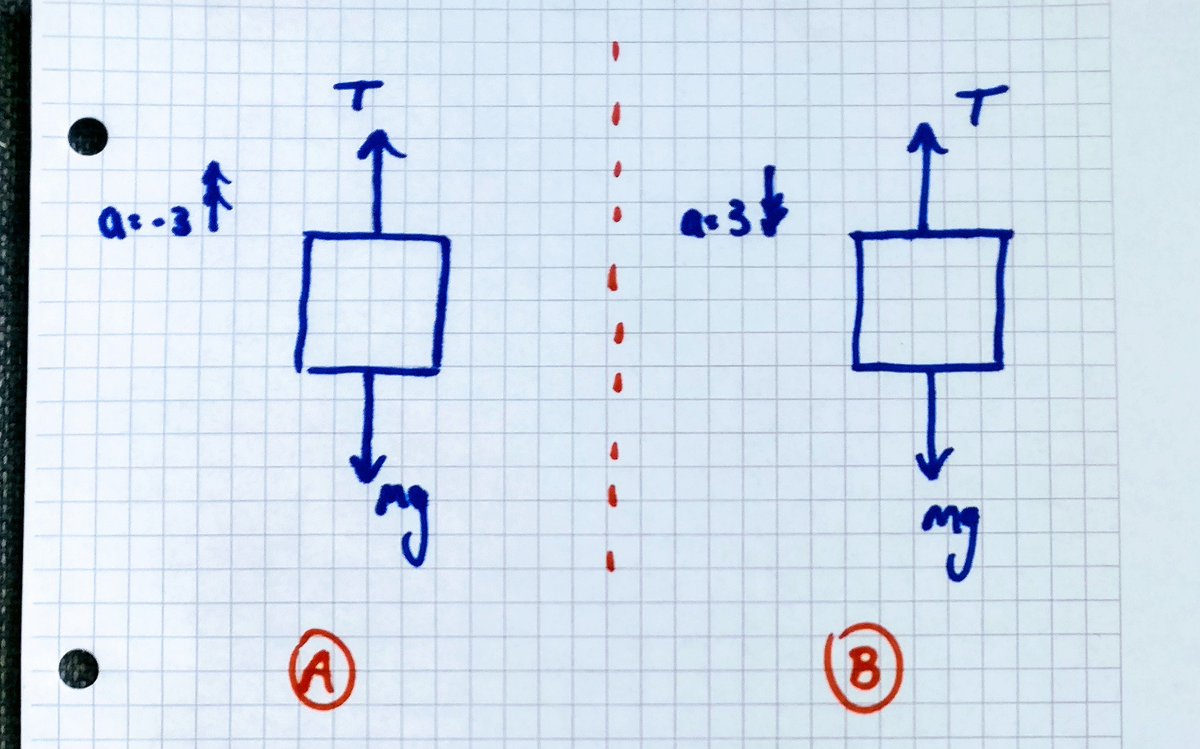
Poll 2: Acceleration Arrows
Time for another mechanics straw poll… A lift is moving upwards but with a deceleration of 3m/s². How would you show this in your diagram?
A very common student misconception in Mechanics is that the direction of acceleration matches the direction of movement. However, wherever possible, I think it makes sense to draw the acceleration arrow to match the direction of motion and this goes hand in hand with interpreting ‘deceleration’ to mean a negative acceleration.
If you show students (or teachers) the diagrams above without any context, our initial intuition would be to think of A as travelling upwards but slowing, and B as travelling downwards and getting faster. Of course, either of the diagrams could match either of those situations and we wouldn’t know which until we were given some information about the object’s velocity.
My main point
Neither is incorrect, but wherever possible I try to draw diagrams in a way that appeals to our intuitive sense of what is happening. (And never deduce the direction of motion from a force diagram!)
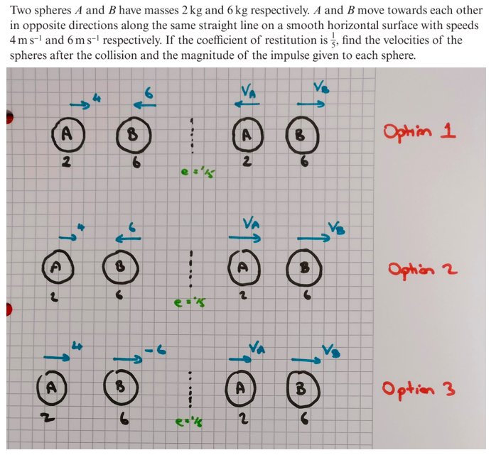
Poll 3: Collisions
Which diagram matches the directions that you would draw the velocity arrows?
I’ll be honest here, and I admit that deliberately I included Option 1 as a bit of a red herring. Following on from the idea of intuition in the last poll, it’s perfectly reasonable to consider that the particles might travel in opposite directions after the collision, but in fact they don’t. Of course, we don’t know this for certain until we’ve solved the equations and we just get a good diagram drawn and then trust in maths to get the signs right for us at the end. I think one risk with Option 1 is if all students get the ‘speed of separation’ correct, but maybe I should have more faith.
I think collisions is the one area where I haven’t fully made up my mind and part of the purpose of this poll was to gauge a majority opinion and to see if that would make me reconsider my own view.
My approach to teaching this topic over the past few years has been to use Option 3: drawing all of the velocity arrows in a common direction, and then assigning them negative values if we know a particle is travelling in the opposite direction. My reasoning is that this helps get signs correct in the conservation of momentum equation and, moreover, I teach the restitution equation symbolically as
rather than using the phrasing ‘speed of separation’ and ‘speed of approach’.
I’m conflicted because this plays along the lines of giving students a single all-purpose method (as discussed with Newton II above) but somewhat goes against the idea of drawing a diagram that matches our intuition (as discussed with acceleration arrows above).
My main-ish point
I really am torn here. I think I’ll continue to teach Option 3, with consistency winning over intuition. (To be honest, some days I’m just glad students draw diagrams at all!) I’m very willing to debate this one further though.
In summary…
Prioritise consistent approaches to solving a whole class of problems, reducing the number of methods students have to learn
As far as possible, draw diagrams to match intuition (but don’t apply the converse and assume a diagrammed system is behaving as you intuit!)
We all nag students to draw good diagrams and to label their equations. It took me a long time to figure out that I should isolate these skills in tests if I really want students to take notice. (Eg give the setup for a full mechanics problem, but only ask for a force diagram; or provide a force diagram and ask for a labelled system of equations (and for them to remain unsolved); or even, present the diagram and the equations and simply ask students to insert the appropriate labels.) In short, if you want them to develop a specific good habit, then test them on that specific good habit!
A footnote on Newton II
Of course, we could argue that F=ma is a special case restricted motion in one-dimension and we should write F=ma and deal with vectors. But then this is a special case, assuming that a is constant so we should write F=m dv/dt. But then this is a special case that assumes the mass is constant, so we should write F=d(mv)/dt.
How do I reconcile this with my approach to consistency and teaching a single method for a whole class of problems? Well, up to (old spec) Mechanics 2 student don’t meet situations with varying mass etc so there’s no need for that extreme generality. It is always nice to discuss it in passing though, especially once they’ve learned about separable differential equations.
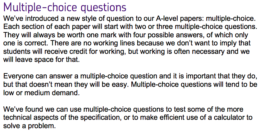
There appears to have been a period roughly during the 1980s when multiple choice questions (MCQ) featured prominently in A-level exam papers. Precisely when or why they appeared and, indeed, when or why they disappeared again is a mystery to me at the moment. Moreover, the only textbooks I’m aware of that include MCQs are those authored by Bostock and Chandler. (There are also a couple of exam preparation books by Shipton and Plumpton that include them: Multiple Choice Tests in Advanced Mathematics, and Examinations in Mathematics.)
In the new A-level
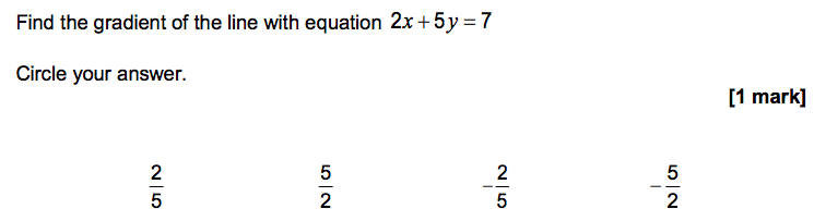
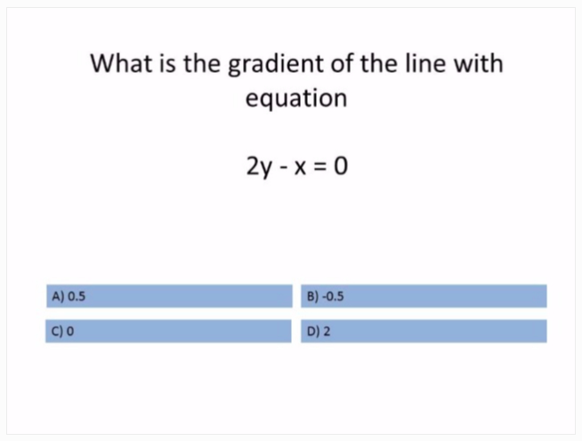
MCQs do get a cameo role in the new A-level assessments from AQA. Each of their Specimen papers includes a couple of MCQs worth a single mark each. Here’s an example from Paper 1:
positioning MCQs as one of four features “at the heart of our aims for the qualification”. Later in the document comes some elaboration:
Aside from ease in assessment terms, I’m keen to focus on the pedagogical value of MCQs and the potential for their use in teaching. The above example feels similar to those offered on the Diagnostic Questions site although I would suggest different potential answers if I wanted to uncover misconceptions (for example, including 2 as an option to identify students who simply observe the coefficient of x).
Diagnostic Questions
Indeed, here is such an MCQ on gradient from the Diagnostic Questions site [sign-in required when following that link]:
One of the excellent features of the Diagnostic Questions is the “insights” where you see students’ explanations for their answers. For example, this student offers their reasoning for (incorrectly) choosing option B:
It’s an MCQ, Jim, but not as we know it
In the 1980s A-level papers, MCQs were a much more serious affair. For a start, there were five different types of MCQ. Even interpreting the instructions is no mean feat. I’ll describe each type and then include an example. [Photos from Plumpton & Shipton.]
Section I (multiple choice)
There is a single correct answer among five options.
Example
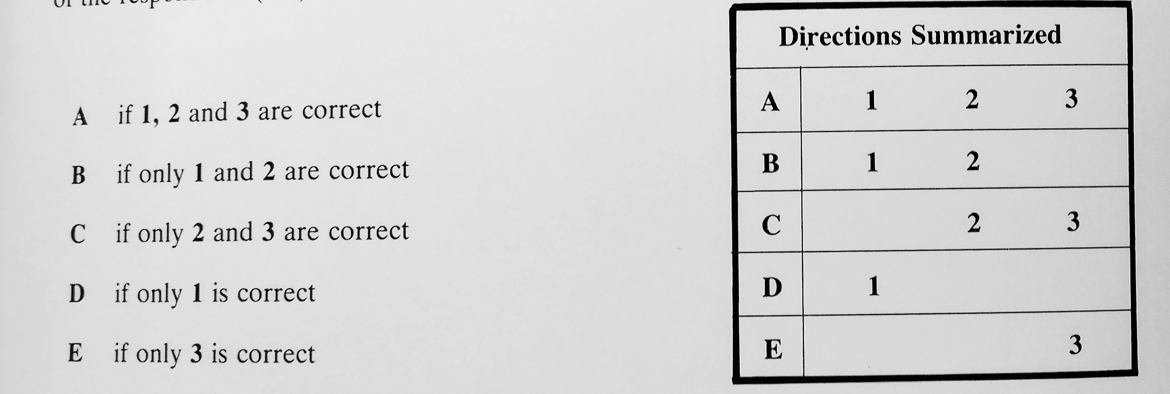
Section II (multiple completion)
Three responses are given (1, 2, 3) of which one or more are correct. The letter representing the student’s answer depends on which are correct:
Example
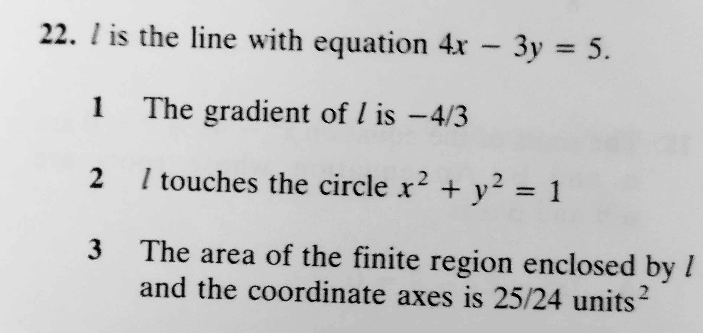
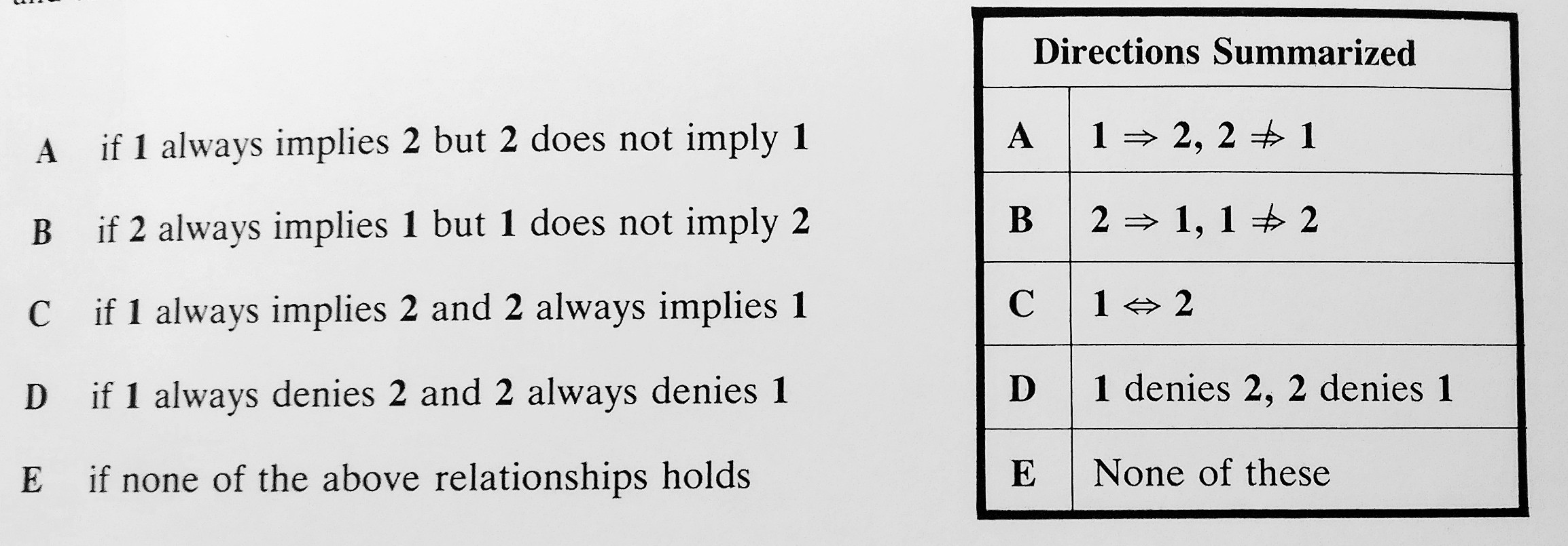
Section III (relationship analysis)
These questions comprise two statements (1 and 2) and the student has to determine the logical relationship between them:
Example
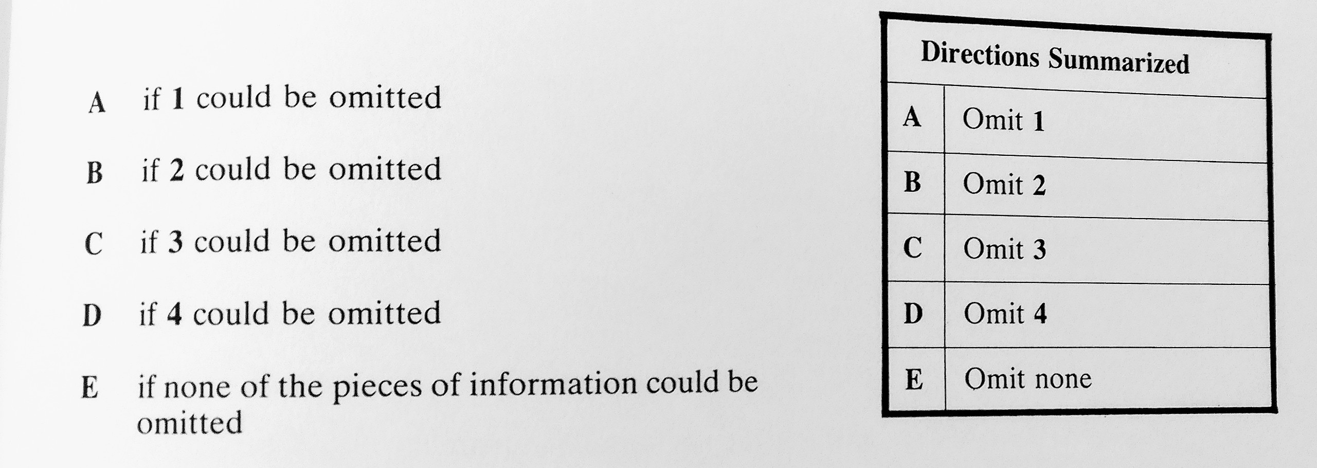
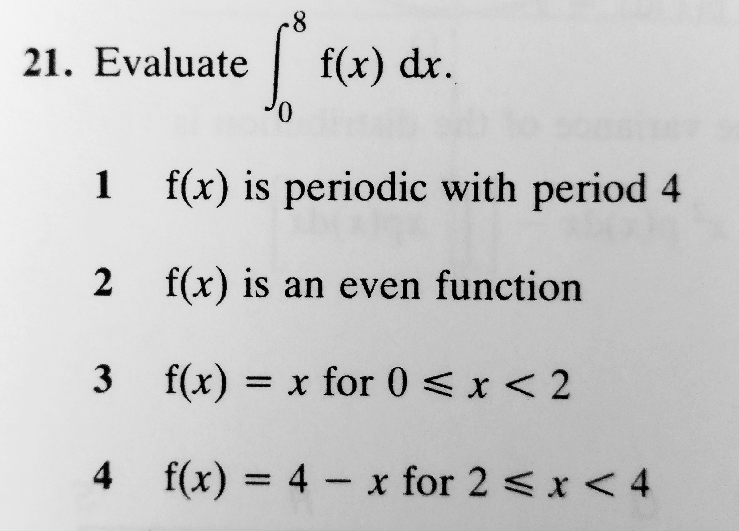
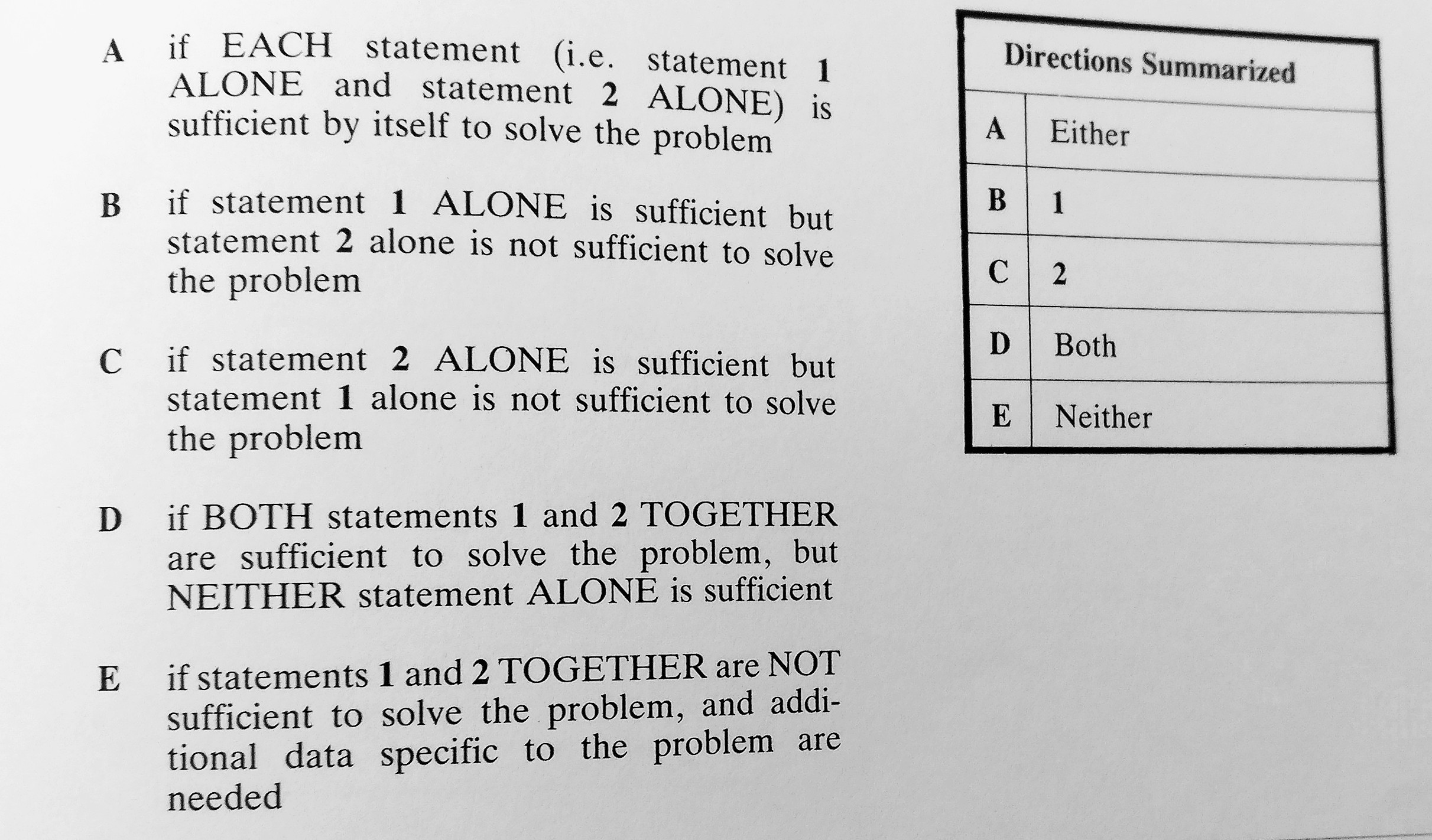
Section IV (data necessity)
A problem is followed by four pieces of information and the student must determine which (if any) piece of information could be omitted and the problem still be solvable:
Example
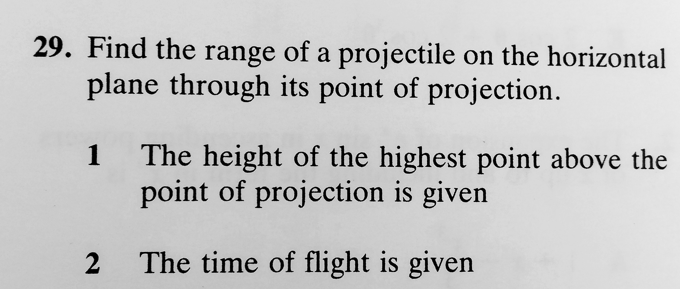
Section V (data sufficiency)
These comprise a problem and two statements (1 and 2) in which data are given. The student has to decide if the given data are sufficient for solving the problem. Brace yourself…
Example
Just a couple more variants…
In Core Maths for A-level, Bostock & Chandler simplify things down to three types:
Type 1: exactly as Section I above
Type 2: akin to Section II above but students simply write the letters corresponding to which items follow from the information in the question.
Type 3: true/false
In their Further Pure Mathematics book, they have:
Types 1 and 2 as in their other text
Type 5 is true/false (as Type 3 in their other text)
Type 3 corresponds to Section III above
Type 4 is an amalgamation of Section IV and Section V: a problem is introduced followed by a number of pieces of information. Either all the information is needed (answer A); the total information given is insufficient (answer I); or some information can be omitted without affecting the solution of the problem (the letters for these items must then be specified)
Use of MCQs in Teaching
I think there is good potential for the use of these more sophisticated MCQs in A-level teaching, although I fear students will either need simplified instructions (for example those used in Bostock & Chandler, rather than the London board papers of the 1980s) or significant training in how to respond. In particular, I agree with Plumpton & Shipton’s comments about Sections III – V:
These items enable coverage of topics which are difficult or unfair to examine by longer structured questions. Indeed, these more sophisticated item types are a far better test of mathematical understanding than some longer questions in which candidates may be applying a method or technique which they have learnt but not have properly understood.
Time to begin building a usable bank of these questions so that I can try them out next year!
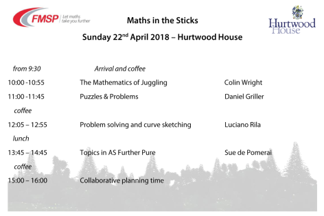
We are now delighted to confirm that “Maths in the Sticks” will be running again this year, on Sunday 22nd April 2018. Many of you will now be familiar with the routine: an engaging day of KS5 professional development with a hearty Sunday lunch! I am also very pleased that we have once again partnered with the Further Maths Support Programme to run this year’s event.
Programme for the Day
All our speakers are now confirmed, though the precise timings of the day may be subject to change.
Our opening speaker this year will be Colin Wright (@colinthemathmo) with his hugely engaging talk on the mathematics of juggling. We are also pleased to welcome Daniel Griller (@puzzlecritic), author of the puzzle book Elastic Numbers, and Luciano Rila (@drtrapezio) from UCL who frequently runs sessions for both A level students and teachers. This year we also have Sue de Pomerai (@suedepom) from the FMSP who will be looking at some of the newer (or at least less familiar) content in the new Further Maths pure module.
Sunday Roast
I have blogged before how CPD really shouldn’t be about the food, but hosting this event on a Sunday was a deliberate decision. Our school serves a roast lunch buffet-style, along with a salad bar and vegan options. I should be able to get a bottle of wine or two open, too!
Hurtwood House
The event will take place at my school, Hurtwood House. Our postcode is RH5 6NU and, as you will see from Google Maps, we are in quite a remote location in the beautiful Surrey hills. Direct access to the school is only possible by car and, where possible, I would encourage people to drive and/or car share. However, so as not to exclude anyone, I can arrange for a minibus pick-up from Guildford train station at 9am. There is a box on the registration form where you can indicate if you would like this service. (Please check that suitable trains run on a Sunday for you to make it to Guildford before 9!) Of course, there will be a return minibus, departing Hurtwood House between 3 and 4pm at the end of the day.
Please also bear in mind that there is a flight of outdoor steps between the room we are using and the canteen. If you are keen to attend but are concerned about accessibility, then please contact me directly and we can see what arrangements might be possible.
Registration
We typically have space for around 35 teachers each year. Please complete the registration form on Eventbrite to book your place.
Job Vacancy – now closed
You might also be interested to know that we are currently advertising a position for a Maths Teacher to join us at Hurtwood. Full details are on our school website here, and the vacancy is also listed on the TES here. (Closing date 2nd February.)


 and
and  .
.

 from the relevant branch.
 is the product
  , however this is unrelated to the product formula for independent events. Indeed, the events ‘able to construct’ and ‘pass’ are not independent here.
 . In all other cases, they are equivalent!
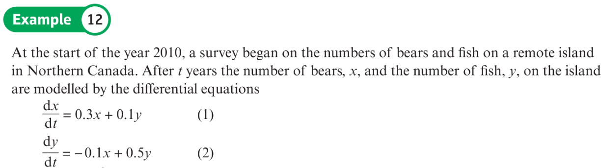


 , where